Conditional formatting for a whole row

A couple of people have recently asked me,

How do I apply the same conditional formatting to all cells in the same row?

The key to this is to use conditional formatting based on a formula.  In the example spreadsheet, Conditional formatting for a whole row, you can find out how this is done but let’s walk through it.

Say we’ve got a budgeting spreadsheet for a business.  In this spreadsheet we have a report that summarises total sales each month against the budget, like so:

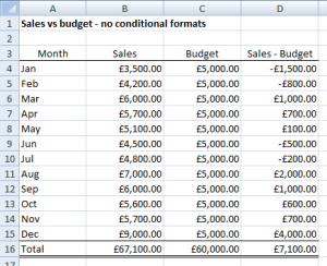
Where we beat the budget we want the whole row to be green, otherwise it should be red.  So where the value in column D is zero or more the whole row should be green.

A Common Mistake

Many people try the following steps:

• Select A4:D16
• Tab across so D4 is the active cell in that range
• Click Conditional Formatting > New Rule
• Select “Format only cells that contain”
• Set up the rule: Cell Value … greater than or equal to … 0
• Change the format to fill the cells with green
• Repeat for a less than zero rule which fills them with red instead.

This works fine for column D, but not A to C.  If you try this you’ll end up with soemthing like this:

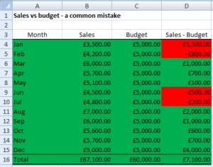
But what’s going on?  Excel is checking each cell’s value against zero.  You haven’t told it that you’re only concerned with column D.  For example, C4 turns green because it’s positive but D4 turns red because it’s negative.

A Solution

Do you think the “Cell Value” rule feels a bit wizard-y?  I do.  We need something that’s a bit more flexible.  One solution is to use a formula instead, like so:

• Select A4:D16
• Observe which row the active cell is on – that’s row 4 in my case..
• Click Conditional Formatting > New Rule
• Select “Use a formula to determine which cells to format“
• In the box underneath enter the following formula: =$D4>=0.  The dollar sign tells Excel it should only be looking at column D.
• Change the format to fill the cells with green
• Repeat for a less than zero rule which fills them with red instead.

And that’s it.  If you do this correctly you should end up with something like this:

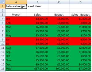
And that’s it!  If want to look into this in more depth then have a look at the example spreadsheet, Conditional formatting for a whole row.

Final Comment

You can apply the same rationale to apply consistent formats to all cells in a column.  Instead of fixing the column in the formula, fix the row number instead.  And so on.

Hope this is useful.  If you have an alternative solution then let me know!