Wipe a memory card

Today I had rather an odd task in mind. I needed to wipe a Compact Flash memory card and be reasonably confident the data was completely gone. Perhaps not usually a task for VBA but it’s what I do quickest so why not?

My idea was simple:

1. Format the drive
2. Write junk data to the drive until it’s full
3. Delete the junk data
4. Format the drive again – for good measure!

Step 2 is the interesting bit. I decided to create a text file (using the VBA Open command) and keep filling it with random numbers until the card was full. Then close it and delete the file.

Now if you try to write data to a drive with no space on it, VBA gets upset! Clearly an error of some sort was bound to happen eventually so I used On Error Resume Next and Application.DisplayAlerts = False to bypass it. Here’s what I came up with:

Sub WipeIt()
    Dim fileNo As Integer
    Const fileName As String = "K:\rubbish.txt" 'junk data file - change as needed
    
    Application.DisplayAlerts = False
    On Error Resume Next
    
    Randomize
    fileNo = FreeFile
    Open fileName For Output As #fileNo
    Do
        Print #fileNo, Rnd()
        If Err.Number  0 Then Exit Do
    Loop
    Close #fileNo
    Kill fileName
    
    On Error GoTo 0
    Application.DisplayAlerts = True
End Sub

Job done!

Reading from and writing to Ranges

VBA developers often need to read data in from Ranges and write results out to other Ranges. It’s a very common task in dashboards for example. The snag is that reading or writing 1 cell at a time can be slow, especially if you have a lot of input or output to deal with. However there are ways to work more efficiently with large tables.

Example 1 – Reading Ranges

Let’s say you’ve need to read some data from A1:A1000 on a worksheet into an array. One way to do this is as follows:

For i = 1 To 1000
    MyArray1(i) = Range("A" & i).Value
Next

However it’s actually very easy to achieve almost the same thing in 1 simple line of code:

MyArray2 = Range("A1:A1000").Value

There is a catch but – in my opinion – it’s a minor one. MyArray2 will actually have 2 dimensions, whereas MyArray1 is constructed with 1. In this example, MyArray2 will have the following bounds:

Dimension 1 ~ 1 To 1000 (representing the row)
Dimension 2 ~ 1 To 1 (single column)

So instead of using MyArray1(i) you now use MyArray2(i, 1). The speed boost can be significant and this next example should help to illustrate the point.

Example 2 – Writing Ranges

Create a blank spreadsheet and coopy the following macro into a blank Module. The idea is that in our code we first do some calculations and store the results in an array. When the code finishes, that array is displayed in cells on a worksheet. Obviously my example calculations are very simple but you could replace them with anything you wish.

Sub test()
    Const rMax As Long = 1000   'total rows
    Const cMax As Long = 100    'total columns

    Dim t As Single     'used to time how long each version takes
    Dim v As Variant    'array containing results of my calculations
    Dim r As Long       'row counter
    Dim c As Long       'column counter

    'This is my "calculation routine" ...
    ReDim v(1 To rMax, 1 To cMax)
    For r = 1 To rMax
        For c = 1 To cMax
            v(r, c) = r + c
        Next
    Next

    'Now let's create the output ...

    'The slow version!
    Cells.Clear
    t = Timer   'start the timer
    For r = 1 To rMax
        For c = 1 To cMax
            Cells(r, c).Value = v(r, c)
        Next
    Next
    MsgBox "Slow version took " & Round(Timer - t, 1) & " seconds"

    'Quick version
    Cells.Clear
    t = Timer   'restart the timer
    Range("A1").Resize(rMax, cMax).Value = v
    MsgBox "Quick version took " & Round(Timer - t, 1) & " seconds"
End Sub

On my PC I got the following messages:

Slow version took 5.4 seconds
Quick version took 0.1 seconds

..see what the comparison is on your machine.

(As a final note, if you do output these results 1 cell at a time then you may not need to store the results in an array at all. I’ve only structured it like this so I can directly compare the time taken creating outputs. In doing so, I hope this illustrates that there are occasions when this might be a good thing to do!)

Repetition

One issue that crops up surprisingly often in spreadsheets is repeating the same calculation.  I see two key problems with this:

1. Inefficiency.
2. Harder to maintain.

Inefficiency

Imagine you didn’t have a spreadsheet.You would never work out the same thing twice, especially if it wasn’t easy! You’d simply find where you had done it before and use it again.

You can do the same thing with spreadsheets. Just store the result in a cell (preferably an appropriately named one) and you can reuse it.

Maintenance

If you duplicate a calculation then you have to maintain every copy of it. Say something changes – perhaps a new parameter is added. Then you might change the calculation in one place but not the other. Or you might make a mistake in one of them. Removing duplication frequently makes it much easier to find and fix errors.

Like so many things it boils down to common sense. Have you experienced spreadsheets like these? Any other top tips? Let me know!

Conditional formatting for a whole row

A couple of people have recently asked me,

How do I apply the same conditional formatting to all cells in the same row?

The key to this is to use conditional formatting based on a formula.  In the example spreadsheet, Conditional formatting for a whole row, you can find out how this is done but let’s walk through it.

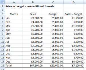
Say we’ve got a budgeting spreadsheet for a business.  In this spreadsheet we have a report that summarises total sales each month against the budget, like so:

Where we beat the budget we want the whole row to be green, otherwise it should be red.  So where the value in column D is zero or more the whole row should be green.

A Common Mistake

Many people try the following steps:

• Select A4:D16
• Tab across so D4 is the active cell in that range
• Click Conditional Formatting > New Rule
• Select “Format only cells that contain”
• Set up the rule: Cell Value … greater than or equal to … 0
• Change the format to fill the cells with green
• Repeat for a less than zero rule which fills them with red instead.

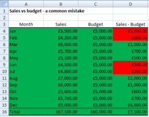
This works fine for column D, but not A to C.  If you try this you’ll end up with soemthing like this:

But what’s going on?  Excel is checking each cell’s value against zero.  You haven’t told it that you’re only concerned with column D.  For example, C4 turns green because it’s positive but D4 turns red because it’s negative.

A Solution

Do you think the “Cell Value” rule feels a bit wizard-y?  I do.  We need something that’s a bit more flexible.  One solution is to use a formula instead, like so:

• Select A4:D16
• Observe which row the active cell is on – that’s row 4 in my case..
• Click Conditional Formatting > New Rule
• Select “Use a formula to determine which cells to format“
• In the box underneath enter the following formula: =$D4>=0.  The dollar sign tells Excel it should only be looking at column D.
• Change the format to fill the cells with green
• Repeat for a less than zero rule which fills them with red instead.

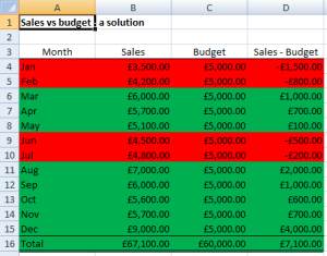
And that’s it.  If you do this correctly you should end up with something like this:

And that’s it!  If want to look into this in more depth then have a look at the example spreadsheet, Conditional formatting for a whole row.

Final Comment

You can apply the same rationale to apply consistent formats to all cells in a column.  Instead of fixing the column in the formula, fix the row number instead.  And so on.

Hope this is useful.  If you have an alternative solution then let me know!

References

There are a lot of people who write add-ins for Excel, myself included.  On several occasions I wondered if I could use those add-ins within the VBA of another spreadsheet.  And of course you can using – you guessed it – references!  And frankly I think references are one of the most criminally under-documented features of VBA in general.I think of references essentially as “VBA add-ins”.  However references are somewhat more powerful add-ins because there is such a variety of things you can use, including things that come built in with Windows or Office.  I’ll give you a couple of examples in a bit.Firstly to have a look at references you need to remember the Tools – References menu option in VBE. This will bring up a huge list of available things you can reference.  In any spreadsheet there are a few standard ones that are ticked at the very top like the “Microsoft Excel Object Library”. I’d recommend that you don’t remove any of these standard ones as they are fundamental to smooth operation.

All the references that you’ve selected will appear at the top of this huge list, with ticks next to them. So you won’t ever need to search the whole list for an elusive tick!

What references might you want?  Well one that I use regularly is the Microsoft Scripting Runtime. This gives you access to the Visual Basic Scripting Object Model, with notable inclusions the Dictionary object and the FileSystemObject.

• Dictionary objects are very similar to Collections  in VBA but with some useful additional features.  If you want to check if an item exists in your Dictionary object then use the Dictionary.Exists method.  And Dictionaries also provide you with a list of the unique IDs of its elements using the Dictionary.Keys property.
• FileSystemObject is a very powerful tool in scripting. You can recurse through Files in a folder or subfolders of a parent folder, create and delete folders and files, check if folders and files exist and so on.  It’s an extremely powerful tool – I may well do a future post dedicated to it.

Another reference I’ve used recently is the CAPICOM Type Library.  I needed a hash function to help me validate some data, so decided to use the MD5 algorithm.  (If you don’t know what a hash function is, it’s essentially just a fancy checksum but it works on text data as well.)  Adding the CAPICOM reference gives you the HashedData object, which can be used to generate a variety of hash functions.

As mentioned at the top, you can even create references to other Excel addins, giving you access to all the same functions and macros.  This can make for some helpful ways to organise and simplify code.

All in all references are an extremely powerful tool and well worth getting acquainted with.  If you’re interested in investigating the Microsoft Scripting Runtime further then I’d also recommend checking out the VB script pages at http://www.devguru.com for a handy reference.

ByVal and ByRef

A few people have asked me what the difference between ByVal and ByRef actually is. In a nutshell it’s the difference between creating a new variable (ByVal) and rebadging an existing one (ByRef).  Here’s an example of some code you can run:

Option Explicit

Public Sub Test()
    Dim x As Double
   
    x = 1
   
    AddTwoByVal x
    Debug.Print x
   
    AddTwoByRef x
    Debug.Print x
End Sub

Private Sub AddTwoByVal(ByVal Value As Double)
    Value = Value + 2
End Sub

Private Sub AddTwoByRef(ByRef Value As Double)
    Value = Value + 2
End Sub

Paste this into a blank module and run the “Test” macro.  You should see the following output in the Immediate Window (press CTRL+G to bring it up if it’s hidden):

1
3

But what’s going on?

Using ByVal creates a whole new variable.  VBA takes the value of x and stores it in a new variable called “Value”.  When AddTwoByVal finishes the variable Value is thrown away along with everything you’ve done to it, so there’s no effect on “x” in Test.

Using ByRef effectively relabels an existing variable.  So in AddTwoByRef you are actually using the same variable as in Test but, figuratively speaking, you’ve stuck it in a box labelled “Value”.  Therefore when AddTwoByRef finishes the changes to “Value” will also be reflected in “x”.

If you don’t specify ByVal or ByRef then VBA assumes ByRef.

You can use this in all sorts of ways. One common application is to address some of the weaknesses of Functions. Functions return a single value (which could be an object or  user-defined type) but what if you want to amend 2 or more values?  Simply create a Sub with the “answers” as arguments passed ByRef – neat trick!

Long Formulae

My number one rule for spreadsheets is a simple one:

A long formula is a bad formula.

Long formulae are the bane of spreadsheets. On more than 1 occasion I have been tempted to write to Microsoft and ask them to impose a 100 character limit on formula length (or at least provide such an option). But what is the problem?

Let’s look at this the other way round for a moment. How many short formulae do you see that are difficult to understand after a little thought? I’ll bet not many. Maybe there’s a new function you need to look up in Excel help but that’s about all. A long formula can suggest many things:

• There are lots of parts to a single calculation.
• A simple calculation is being performed in an overly complicated way.
• The author is basically showing off (frankly the worst crime of all!)

For sake of illustration I’m going to calculate a person’s Body Mass Index (BMI).  BMI is defined as:

BMI = (Weight in kilograms) / (Height in metres) ^ 2

My spreadsheet is reasonably flexible. It allows people to choose the units they use for entering height and weight. Height can be entered in metres or feet. Weight can be entered in kilograms, stones or pounds. (I’m assuming that users are capable of entering fractions, e.g. 10 stones 6 pounds would be entered using =10+6/14.)

B1 = height value
C1 = height units (“metres” or “feet”)

B2 = weight value
C2 = weight units (“kilograms”, “stones” or “pounds”)

To calculate BMI in one go you could use this formula:

=B2*IF(C2=”kilograms”,1,IF(C2=”stones”,1/0.1575,1/2.205))/((B1*IF(C1=”feet”,1/3.281,1))^2)

This isn’t too bad but it could definitely be easier to follow! Think about how you would check it. You would probably have to break it down as follows and check each part somehow (e.g. using ‘Evaluate Formula’ and stepping through a couple of example calcs):

1. Convert height into metres
2. Convert weight into kilograms
3. Calculate BMI

Surely it would be clearer if these steps were shown separately?

Let’s say we put the height in metres in cell B4. To convert to metres we just pick out this part:
=B1*IF(C1=”feet”,1/3.281,1)

Now let’s put weight in kilograms in cell B5. Now we just pick out this part:
=B2*IF(C2=”kilograms”,1,IF(C2=”stones”,1/0.1575,1/2.205))

Finally the BMI formula goes from that first formula above to something that resembles the definition much more closely:
=B5/B4^2

Notice how much easier this is to check too.  You can easily check that each conversion is working correctly. Then checking the BMI formula itself is simplicity itself!

IFERROR – a new(ish) way to handle errors

Oftentimes I see formulae that attempt to deal with errors, such as division by zero or failed VLOOKUPs.  Something like this for example:

=IF(ISERROR([something]),[something else],[something])

I never liked this because Excel actually has to do the [something] bit twice. Worse yet you may get one right and one wrong, e.g. due to updating one but not the other. Excel 2007 introduced a new function that addresses these points, called IFERROR. The following formula does exactly the same as the above but more robustly:

=IFERROR([something],[something else])

If [something] returns a valid answer then IFERROR returns it! If it’s an error then IFERROR will return the result of the [something else] calculation instead. Notice how much shorter the formula can be, especially if [something] is quite long. Plus you only have to type each part once so there’s less risk of accidents.

As a final point do beware of sending the spreadsheet to anyone using an earlier version of Excel. If you do then this function won’t be recognised and you’ll just get errors! In such cases you may need to rewrite these formulae using the original format shown above. Alternatively you can easily recreate the IFERROR function in VBA instead – just paste the following into a module:

Public Function IfError(Value, OtherValue)
‘Do not use this if saving in Excel 2007 format or later!
    If IsError(Value) Then IfError = OtherValue Else IfError = Value
End Function

Use Print Preview!

Easy one, this! To put it succinctly, get into the habit of looking at Print Preview.

You’ve written a spreadsheet and next job is to pass it on to a colleague to have a look. Before you do anything else, have a quick look at Print Preview.  A lot of people will automatically print everything out that you send to them – documents, pictures, spreadsheets, you name it.  Now I’m not going to be an eco-warrior here – the rights and wrongs of this are not the point.  The point is that in the real world and that’s what (some) people do.

Now I don’t know about you but I’m certain that my boss wouldn’t be very happy if I handed him a spreadsheet and he ended up sending 100 pages to the printer, 90 of which were junk.  It really is that simple.  A quick look a Print Preview can save you a lot of (easily avoided) headaches!

On top of that Excel provides something called “Page Break Preview”, which appears on the “View” tab in Excel 2007.  This gives you a visual guide to where all the page breaks will appear when you print it.  The dashed lines are where Excel has put a page break for you, the solid ones are added by hand.  You can drag these around as needed.  When you’ve finished switch back to “Normal” view and you’re done.  A small investment of time goes a long way!

Overwritten Cells

Very often where I work I come across spreadsheets of a certain type, characterised as follows:

• 1 row containing headings (of varying levels of helpfulness) …
• followed by 1 row containing formulae …
• all copied down for several hundred rows or more.

This is the kind of thing that spreadsheets are really good at. Write your calculations for 1 record and copy them as many times as you need. Brilliant.

That’s all fine as long as people don’t mess it up! All too often I see situations where the formula in cell AZ653 doesn’t quite work due to a quirk in that record. Rather than think about the wider implications the user simply types the right value in instead and carries on regardless. There are numerous problems with this but I’ll concentrate on the poor person whose job it is to check this spreadsheet. It is very possible that this change will be missed, or perhaps just become overwritten, e.g. if someone copies all the formulae right the way down again. We need an easy way to spot it.

Enter column differences. First select the range containing all the formulae but leave out the header row(s). In Excel 2007 the command is found here:

• Home tab
• Find & Select
• Go To Special
• Select the “Column differences” option
• Press OK.

(A slightly quicker route is to press the F5 key followed by the “Special” button.) Now Excel will only select those cells where the formulae don’t match with those in the first row. You can cycle through these cells by pressing the TAB key. You can even colour the cells in using the normal fill control.

This works equally well when you have lots of formulae in a column copied across to the right. Only this time – you guessed it – you would select “Row differences” instead.

These range differences are powerful tools that can be a real life saver. If you ever come across spreadsheets like the ones I’ve described then I heartily recommend getting used to using these tools.